GPU programming part 3: a partial real-world example

As promised last time, in the third and final installment we would look at some actual code. As it will turn out, our straightforward implementation will need a little rework in order to properly fire up the GPU.

An algorithm example

As an illustrative example, let’s consider a part of the t-SNE algorithm. We will quickly introduce some of the mathematics behind the algorithm. This background is not needed to understand the actual coding part, so the not-so-mathematically inclined reader can skip right to the code part.

The t-SNE algorithm is used to visualize high-dimensional data in two or three dimensions. Such data is quite common in the machine-learning and AI world, where symbols (e.g. words, parts of audio or images etc.) are mapped to high dimensional vectors. These vectors can easily reach up to hundreds of components, making it almost impossible to intuitively grasp how the data is distributed. When doing data analysis and statistics, one of the cardinal rules is that you should always do some inspection of your data before analysis too see if you can spot some patterns or anomalies. If possible, such analysis should include a visual data representation, as single number metrics can easily paint a deceitful image of the statistical distribution.

The t-SNE algorithm basically tries to find a mapping to a lower dimensional representation of the high dimensional sample, such that the two distributions are as similar as possible. It does this by trying to minimize the statistical distance of the observed distribution $P$, and the low-dimension target distribution for visualisation $Q$, using by the Kullback-Leibler divergence, which is defined as

$$KL(P \, || Q) = \sum_{i \ne j} p_{j|i} \log_2 \frac{p_{j|i}}{q_{j|i}}$$

This is actually quite a common loss function in different machine learning tasks. Here $P$ is a derived property distribution from the actual sample, and $Q$ is derived from the distribution we want to find.

To make matters not to complicated, we will focus only on computing the sets of $p_{j|i}$. These only need to be computed once, since they are a property of the static input data. They are given by

$$p_{j|i} = \frac{ \exp(- \| \vec{x}_i - \vec{x}_j\|^2 / \sigma_i ) }{ \sum_ {k \ne i} \exp(- \| \vec{x}_i - \vec{x}_k\|^2 / \sigma_i )},$$

where the vertical bars denote the "length" of the vector. The equation gives a weighted distribution of the distances between the vector entries $\vec{x}$. In the algorithm, we would have to find a scaling parameter $\sigma_i$, but we will not be concerning ourselves with that, either. Instead, we will look at computing the distances between all possible vector pairs $\vec{x}_i$ and $\vec{x}_j$, as these have to only be computed only once and can be cached.

We note that the distance of a vector to itself is zero, and that the differences function is symmetric, so we only have to compute half of all the permutations. In math terms, it means we have a symmetric matrix.

The code

With the math out of the way, lets do some programming. For brevity, we’ll skip the boilerplate code to reading the file, and concentrate on the CUDA code only, since that is not the topic for today.

As our data source, we use a vector file with 16384 entries of length 300. The vectors will be laid out sequentially in memory, since that is the format they come in from the csv file.

To map the indices $i$ and $j$ to a linear index on our triangular matrix, we use this nifty transformation^[1]:

__device__ int2 lin_to_triu(int t_off, int nx)
{
    int i = nx - 2 - floorf(sqrtf(-8 * t_off + 4 * nx * (nx - 1) - 7) / 2.0 - 0.5);
    int j = t_off + i + 1 - nx * (nx - 1) / 2 + (nx - i) * ( (nx - i) - 1) / 2;

    return {i, j};
}

For a linear index t_off, it will return a pair of indices such that we can iterate over all combinations of vectors for a vector set of size nx. We don’t have to cache the case $i = j$, since the distance of a vector to itself is trivially 0.

CUDA supports short vectors of primitives, such as int2, which we use to our advantage here.

For our example, suppose we have our data in a buffer

float *input_data = read_input_from_file();

The input_data variable is a pointer in memory that we need to provide to the CUDA driver to copy our data to the system. When allocating memory for data to be copied to the CPU, a developer needs to decide whether to use a regular or a pinned buffer. A pinned buffer is a memory region whose physical address cannot be changed or by swapped to disk, and should be in a region that is reachable by the GPU’s Direct Memory Access controller. Such memory regions are typically scarcer then other memory regions, so we have to prudent when claiming them. On the other hand, if we use a regular memory region, the CUDA driver will copy that data to a temporary pinned buffer first and deletes it after the copy is complete. So, we could just as well claim such region directly as we can release it back after the copy to device is finished.

Next, we need to copy this data to the GPU. This is done by

static float *copy_input_to_gpu(const float *data, int nx, int xlen)
{
    float *d_x_in;
    size_t d_x_in_size = nx * xlen * sizeof(float);

    // allocate memory in device memory, and verify that the allocation was successful
    auto err1 = cudaMalloc(&d_x_in, d_x_in_size);

    // always check the status of calls into the CUDA SDK
    if (err1 != cudaSuccess)
    {
        throw std::runtime_error(fmt::format("Error allocating GPU memory for source data: {}, {}", cudaGetErrorName(err1), cudaGetErrorString(err1)));
    }

    // copy data from RAM source to device memory destination, and verify copy was successful.
    auto err2 = cudaMemcpy(d_x_in, data, d_x_in_size, cudaMemcpyHostToDevice);

    if (err2 != cudaSuccess)
    {
        throw std::runtime_error(fmt::format("Error copying source data to GPU: {}, {}", cudaGetErrorName(err2), cudaGetErrorString(err2)));
    }

    return d_x_in;
}

It is customary to denote pointers to device memory with the d_ prefix, as they cannot be released with the regular free() memory release method. Off course, in a production environment this resource management would be tied to a class constructor and destructor to guarantee proper memory release.

Great, we now have the input data in the GPU’s memory, so we can call the actual kernel. A straightforward implementation would look something like this:

__global__ void
diff_x_matrix_triu(const float *__restrict__ xarr,
                   float *__restrict__ xdiff,
                   int nx,
                   int xlen)
{
    int t_off = blockDim.x * blockIdx.x + threadIdx.x;

    if (t_off < triu_max_dev(nx))
    {
        int2 indices = lin_to_triu(t_off, nx);
        int i = indices.x;
        int j = indices.y;

        float acc = 0.;
        for (int k = 0; k < xlen; k++)
        {
            acc += powf(xarr[i * xlen + k] - xarr[j * xlen + k], 2);
        }

        xdiff[t_off] = acc;
    }
}

The __global__ attribute tells the compiler that this GPU function should be callable from the host. The __restrict__ attribute is not strictly necessary. It tells the compiler that the pointers cannot alias, meaning that writing to xdiff cannot change the data read through xarr, enabling some optimizations. We developers are then responsible to upholding that contract; we promised the compiler it will not happen. Last, we need to provide the size of the input data, as it cannot obtained from the pointer arguments.

This kernel can be launched with a simple helper routine such as

// return the number of elements in a triangular matrix without the diagonal
int triu_max_cpu(int nx)
{
    return (nx * (nx - 1)) >> 1;
}

void run_kernel_wrapper(int nx, int xlen, float *d_vectors, float *d_distances) {
    // arbitrarily chosen multiple of 32
    dim3 thread_dim = 128;

    // if the input size does not fit our block size exactly, increase
    // the block size by 1 for the last part of the input data.
    dim3 block_dim = triu_max_cpu(nx) / thread_dim.x + (triu_max_cpu(nx) % thread_dim.x == 0 ? 0 : 1);

    // this notation is syntactical sugar for a regular call to the CUDA driver API
    diff_x_matrix_triu<<<block_dim, thread_dim>>>(d_vectors, d_distances, nx, xlen);
}

Remember that we always have to schedule threads 32 at a time (a warp), so it makes sense to have thread_dim a multiple of 32. If not, the CUDA runtime will disable some threads in the last warp to match the block size that otherwise could have done useful work. For convience, the CUDA SDK supports multidimensional block and grid sizes. We have no need for those here. Also, the maximum number of threads is still limited by the architecture generation. For example, I have a somewhat older GPU of compute generation 7.5. This means it has a limit of 1024 threads per block, or 32 warps in total. This generation has a uniquely small amounts of threads per block; most prior and subsequent architecture generations support double that amount.

For our initial implementation, however, it doesn’t really matter. Our warps are not dependent on each other, so we can pick any multiple of 32 and be just fine. We compile our kernel with the nvidia CUDA compiler together with the boilerplate to read the csv, resulting in executable cuda_demo_program. Our program will read our vector data from csv file vec16k_300.csv. We and run the Nvidia Nsight compute profiler with full metric collection (--set full) to see how good our implementation is:

ncu --set full -f -o profile cuda_demo_program vec16k_300.csv

This gives us a profile we can read with the Nvidia Nsight compute to see what happened. In the top of the application, we see a summary overview of the profiling results:

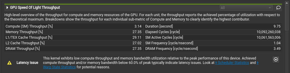
Figure 1. A profile overview of our first kernel attempt.

Well, that is quite underwhelming. The compute throughput is only at 3%. Memory throughput is not exactly stellar with just over 27%, either. We see in the UI there is a suggestion to look at the scheduler statistics to see what is going on. Scrolling down to the sections reveals our issue:

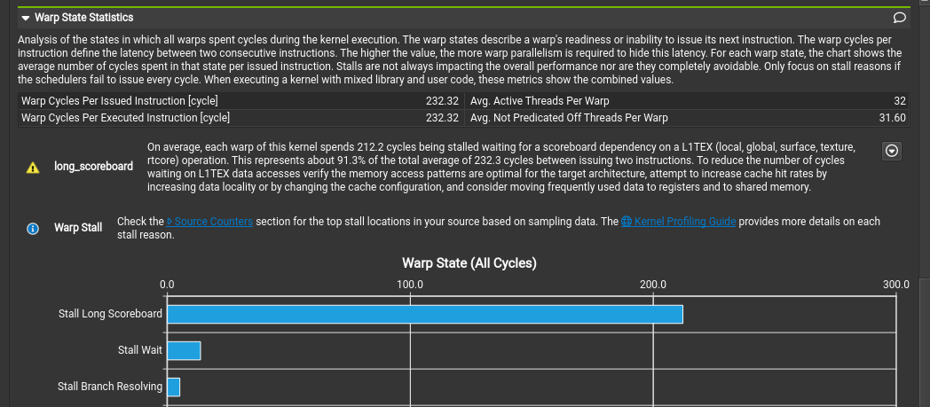
Figure 2. A profile overview of our first kernel attempt.

Most warps are in the Stall Long Scoreboard state most of the time. Any warp that is not in the Selected state will not be executed, and we have a lot of warps that are not selected. Looking in the nSight kernel profiler documentation, we find the smsp__pcsamp_warps_issue_stalled_long_scoreboard warp stall reason. The wording is a bit technical here, but what is basically says is that the data required was not present in cache, i.e. it had to be fetched from slow device memory.

Looking at the instruction counter section, we immediately see the problem:

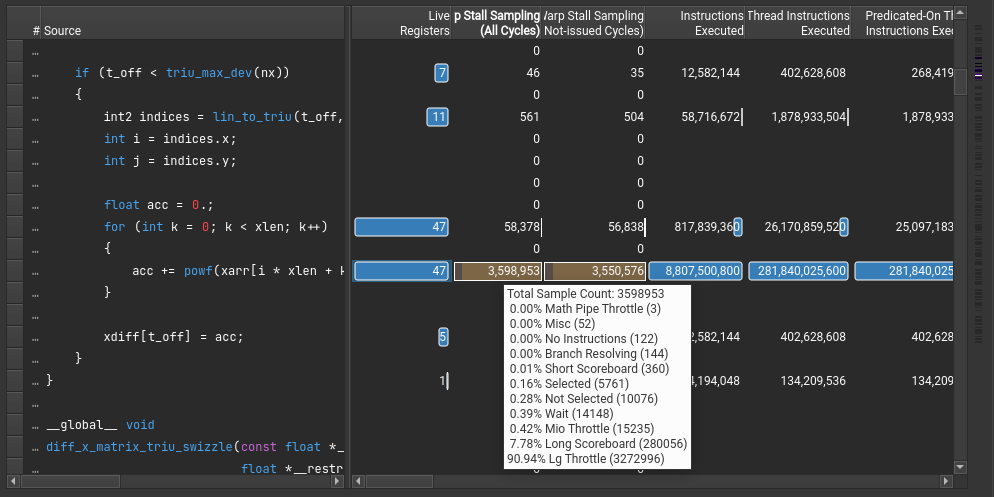
Figure 3. Instruction count and warp stall reasons for our kernel bottleneck.

The loading of data to compute the vector difference is, as we say from the overview, mostly spending its time waiting: only 0.16% of the cycles were used to actually load data or compute something.

As we discussed before, device memory interactions tend to be slow and should be avoided by using shared memory or latency hiding. In our case, there is not much latency hiding we can do, as our operations on the data are quite short; we are memory bound.

That leaves us with the other option, using shared memory. When looking at the workload, we can quickly see that we need to load the same data over and over from global memory. So lets try to bring as much data as possible into shared memory. We load part of the dataset once to shared memory, compute all differences from this subset, and load the next subset.

Unfortunately, shared memory is a scarce resource, particularly in architecture generation 7.5 which I have, being only 64 kb per multiprocessor. Now, we need to do some math to figure out what to do. In this example, we do it by hand, but in a production system you would typically want to automate this parameter computation as the size of your input data is not known beforehand. In our test case, we do know the sizes however, which makes illustrating the trade-offs a bit simpler. Each vector has 300 components of 32 bits single precision floats, so we can load 54 vectors in shared memory per kernel block. Using the binomial coefficient tells us that with 54 vectors, we can make 1431 different pairs. However, our processor only supports 1024 threads per multiprocessor, so we cannot effectively utilize such large subsets, anyway. But we do want to have a large size as possible, as the number of threads we can run grows exponentially with the size of the data subset.

For our example, we will settle at a subset of 32 vectors. This gives us 496 different pairs, which is quite close to 512 threads, or 16 warps. Sadly, this requires more than half of the shared memory for the subset that is available. This means that we can only use half of the scheduler queue capacity, but trade-offs like these happen when doing GPU programming. Besides, not all is lost, since the number of threads that can execute on a multiprocessor is much lower anyway, so we are really "only" giving up some possibilities for latency hiding. To see how bad this will influence our performance we will see when we profile.

For our next code attempt^[2], we also make another change in the data layout. Originally, the vectors were laid out sequentially in memory, but this will lead to problems when copying to shared memory. When accessing shared memory, requests are coalesced but banked. Per request, we can fetch 32 4-byte data elements (such as a single precision float), provided all 32 memory accesses are mapped to different banks. If not, subsequent requests have to be made to memory until all data to maps to the same bank is resolved.

This shows why it is nice to have a subset of 32 vectors. If we transpose the data, we just need 300 128-byte aligned writes to shared memory, eliding bank conflicts when writing and when reading.

Finally, I made another small tweak where we swap the powf function for a regular multiplication. We cut the dataset up in subsets of 16 vectors, leading to 1024 subsets in our case, and each block in our kernel works on a pair of subsets until all subset pairs have been evaluated.

The optimized code now looks like this:

__global__ void
diff_x_matrix_triu_swizzle2(const float *__restrict__ xarr,
                            float *__restrict__ xdiff,
                            int nx,
                            int xlen)
{
    // first, copy in n_shared * 300 items with 512 threads
    std::size_t n_shared = 32;

    // Get the pointer to shared memory from the runtime
    extern __shared__ float xarr_shared[];

    int2 block_offset = lin_to_triu(blockIdx.x, 1024);

    int warp_id = threadIdx.x / warpSize;
    int lane_id = threadIdx.x % warpSize;

    for (int n = 0; n < 19; n++) // 300 components loaded by 16 warps requires 19 rounds
    {
        int row_dst_id = warp_id + 16 * n;

        int offset = lane_id + lane_id < 16 ? block_offset.x : block_offset.y;

        if (row_dst_id < 300)
        {
            xarr_shared[row_dst_id * n_shared + lane_id] = xarr[row_dst_id * nx + offset];
        }
    }

    // wait until all threads are done copying
    __syncthreads();

    int glb_off = blockIdx.x * 496 + threadIdx.x;

    if (glb_off < triu_max_dev(nx) && threadIdx.x < 496)
    {
        int2 indices = lin_to_triu(threadIdx.x, n_shared);
        std::size_t i = indices.x;
        std::size_t j = indices.y;

        float acc = 0.;
        std::size_t kmax = n_shared * xlen;

        for (std::size_t k = 0; k < kmax; k += n_shared)
        {
            float tmp = xarr_shared[i + k] - xarr_shared[j + k];
            acc += tmp * tmp;
        }

        xdiff[glb_off] = acc;
    }
}

There might be a lot to unpack, but the code basically splits in two. In the first half, we copy memory from global memory to shared memory. Each thread can only issue a load for a single data element. The GPU memory controller will try to bundle the requests into one or more wide requests from global memory.

Once a thread is done fetching the data, we need to make sure that all other threads are done with their job loading data as well. That is why we need the __syncthreads(). It is a barrier at the block level, involving all threads that are part of our block.

In the second part, we need to mask out part of the warp. We issues 16 warps, or 512 threads, but there are only 496 jobs in the block, so the last warp has half of its threads silenced. With GPU programming, this kind of suboptimal utilization to fit the problem size is sometimes inevitable, unfortunately. Also, we made some small changes to reflect the changed memory layout.

Okay, we are all done now, so lets fire up the profiler again and see what happens. Nsight compute has a very nice function that we can visualize two or more different profiles against each other, so lets put that functionality to good use:

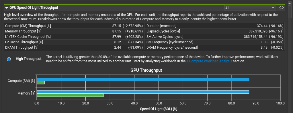
Figure 4. A profile overview of our optimized attempt.

Well, that certainly looks much better. Utilization of the GPU hardware has gone up tremendously. This is reflected in the execution time, which now takes less then 4% of our naive first attempt.

Off course, we want to see if there is more that we have left on the table, so lets check the warp scheduler statistics:

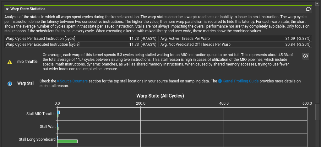
Figure 5. A chart of the stall reasons for our optimized kernel.

It is a bit difficult to see the absolute numbers, since the numbers of our naive attempt where so dismal, but from the order we can infer that the MIO Throtle is the main reason. Checking again the profiler docs, we read that this means the shared memory bus is too busy and cannot keep up with the ALU (the unit that does basic calculations and operations on a processor). These situations could be remedied by keeping data into registers longer. In our situation, this is not possible, however, since we read the data only once per thread. So that means we are pretty optimal right now.

To verify, lets look at the instruction counters for the source code as well:

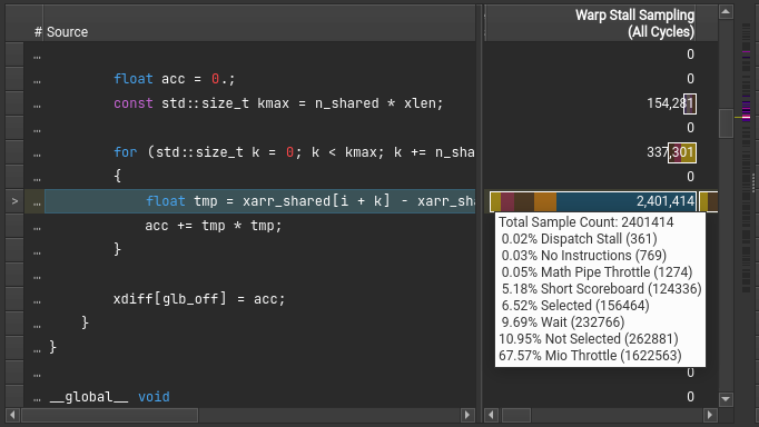
Figure 6. Annotated source code with profiler statistics.

That looks solid. Our top for warp select states are waiting for shared memory, occupied hardware and actually running. To be really sure, we can check the counters on the PTX source as well.

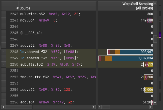
Figure 7. Annotated PTX code with profiler statistics.

PTX is an assembly-like in-between form between CUDA code and the actual GPU assembly code — a bit like e.g. Java bytecode. Compared to the latter, it is extensively documented, so we can get a good idea on what is going on.

The line that we are interested in, the loading of the two data elements and subtracting them, results in just three instructions. This confirms that the shared memory loading is indeed our bottleneck. Interestingly, the metrics between the two load operations (ld.shared.f32) are quite different. I suspect this due to issues mapping the actual assembly counters back to PTX.

To squeeze out even more performance, there is actually a lot of sampling data that we can view. Those samples are not all that relevant, however, so we will not dive into them for today. With the GPU already at 80% compute throughput, the will be diminishing returns for further optimizations that will likely be more complicated in nature, too.

With that, we conclude this example of into bringing computations to the GPU.

We have seen that in order to obtain good performance, we have to take into account the particularities of the GPU model. Partitioning the problem into smaller sub-problems and maintaining a good memory layout were in this case vital for performance, and they very often are in general. While taking these particularities into account provides an additional challenge, it is also a fun and rewarding endeavour.

With a lot of cloud vendors now lending out massive compute power via GPU’s, now is a better time then ever to start using GPU programming.

1. https://stackoverflow.com/a/27088560

2. Actually, I went through many iterations before I came up with the final result :-)